Barrier certificates for collision avoidance

Adapted from: Example 2 of "Engineering applications of SOS polynomials" by Georgina Hall, from the 2019 AMS Short Course on Sum of Squares: Theory and Applications Implementation by: Hugo Tadashi Kussaba

using DynamicPolynomials
@polyvar x[1:2]

using SumOfSquares
using CSDP

We need to pick an SDP solver, see here for a list of the available choices. We use SOSModel instead of Model to be able to use the >= syntax for Sum-of-Squares constraints.

solver = optimizer_with_attributes(CSDP.Optimizer, MOI.Silent() => true)
model = SOSModel(solver);

We define below the vector field $\text{d}x/\text{d}t = f$

f = [x[2], -x[1] + (1/3)*x[1]^3 - x[2]]

2-element Vector{DynamicPolynomials.Polynomial{Float64}}:
 x₂
 -x₂ - x₁ + 0.3333333333333333x₁³

Semi-algebraic function describing the unsafe set 𝒳ᵤ

g₁ = -(x[1]+1)^2 - (x[2]+1)^2 + 0.16  # 𝒳ᵤ = {x ∈ R²: g₁(x) ≥ 0}

\[ -1.84 - 2.0x_{2} - 2.0x_{1} - x_{2}^{2} - x_{1}^{2} \]

Semi-algebraic function describing the initial set 𝒳₀

h₁ = -(x[1]-1.5)^2 - x[2]^2 + 0.25    # 𝒳₀ = {x ∈ R²: h₁(x) ≥ 0}

\[ -2.0 + 3.0x_{1} - x_{2}^{2} - x_{1}^{2} \]

Define SOS barrier function B

monos = monomials(x, 0:4)
@variable(model, B, Poly(monos))

\[ ({\_}_{1}) + ({\_}_{2})x_{2} + ({\_}_{3})x_{1} + ({\_}_{4})x_{2}^{2} + ({\_}_{5})x_{1}x_{2} + ({\_}_{6})x_{1}^{2} + ({\_}_{7})x_{2}^{3} + ({\_}_{8})x_{1}x_{2}^{2} + ({\_}_{9})x_{1}^{2}x_{2} + ({\_}_{10})x_{1}^{3} + ({\_}_{11})x_{2}^{4} + ({\_}_{12})x_{1}x_{2}^{3} + ({\_}_{13})x_{1}^{2}x_{2}^{2} + ({\_}_{14})x_{1}^{3}x_{2} + ({\_}_{15})x_{1}^{4} \]

Define barrier certificate constraints using SOS relaxation

B(x) > 0 for all x ∈ 𝒳ᵤ

ε = 0.001
@constraint(model, B >= ε, domain = @set(g₁ >= 0))

\[ ({\_}_{1} - 0.001) + ({\_}_{2})x_{2} + ({\_}_{3})x_{1} + ({\_}_{4})x_{2}^{2} + ({\_}_{5})x_{1}x_{2} + ({\_}_{6})x_{1}^{2} + ({\_}_{7})x_{2}^{3} + ({\_}_{8})x_{1}x_{2}^{2} + ({\_}_{9})x_{1}^{2}x_{2} + ({\_}_{10})x_{1}^{3} + ({\_}_{11})x_{2}^{4} + ({\_}_{12})x_{1}x_{2}^{3} + ({\_}_{13})x_{1}^{2}x_{2}^{2} + ({\_}_{14})x_{1}^{3}x_{2} + ({\_}_{15})x_{1}^{4} \text{ is SOS} \]

B(x) ≤ 0 for all x ∈ 𝒳₀

@constraint(model, B <= 0, domain = @set(h₁ >= 0))

\[ (-{\_}_{1}) + (-{\_}_{2})x_{2} + (-{\_}_{3})x_{1} + (-{\_}_{4})x_{2}^{2} + (-{\_}_{5})x_{1}x_{2} + (-{\_}_{6})x_{1}^{2} + (-{\_}_{7})x_{2}^{3} + (-{\_}_{8})x_{1}x_{2}^{2} + (-{\_}_{9})x_{1}^{2}x_{2} + (-{\_}_{10})x_{1}^{3} + (-{\_}_{11})x_{2}^{4} + (-{\_}_{12})x_{1}x_{2}^{3} + (-{\_}_{13})x_{1}^{2}x_{2}^{2} + (-{\_}_{14})x_{1}^{3}x_{2} + (-{\_}_{15})x_{1}^{4} \text{ is SOS} \]

Ḃ(x) ≤ 0 for all x ∈ R²

using LinearAlgebra # Needed for `dot`
dBdt = dot(differentiate(B, x), f)
@constraint(model, -dBdt >= 0)

\[ ({\_}_{2} - {\_}_{3})x_{2} + ({\_}_{2})x_{1} + (2 {\_}_{4} - {\_}_{5})x_{2}^{2} + (2 {\_}_{4} + {\_}_{5} - 2 {\_}_{6})x_{1}x_{2} + ({\_}_{5})x_{1}^{2} + (3 {\_}_{7} - {\_}_{8})x_{2}^{3} + (3 {\_}_{7} + 2 {\_}_{8} - 2 {\_}_{9})x_{1}x_{2}^{2} + (2 {\_}_{8} + {\_}_{9} - 3 {\_}_{10})x_{1}^{2}x_{2} + (-0.3333333333333333 {\_}_{2} + {\_}_{9})x_{1}^{3} + (4 {\_}_{11} - {\_}_{12})x_{2}^{4} + (4 {\_}_{11} + 3 {\_}_{12} - 2 {\_}_{13})x_{1}x_{2}^{3} + (3 {\_}_{12} + 2 {\_}_{13} - 3 {\_}_{14})x_{1}^{2}x_{2}^{2} + (-0.6666666666666666 {\_}_{4} + 2 {\_}_{13} + {\_}_{14} - 4 {\_}_{15})x_{1}^{3}x_{2} + (-0.3333333333333333 {\_}_{5} + {\_}_{14})x_{1}^{4} + (-{\_}_{7})x_{1}^{3}x_{2}^{2} + (-0.6666666666666666 {\_}_{8})x_{1}^{4}x_{2} + (-0.3333333333333333 {\_}_{9})x_{1}^{5} + (-1.3333333333333333 {\_}_{11})x_{1}^{3}x_{2}^{3} + (-{\_}_{12})x_{1}^{4}x_{2}^{2} + (-0.6666666666666666 {\_}_{13})x_{1}^{5}x_{2} + (-0.3333333333333333 {\_}_{14})x_{1}^{6} \text{ is SOS} \]

The model is ready to be optimized by the solver:

JuMP.optimize!(model)

We verify that the solver has found a feasible solution:

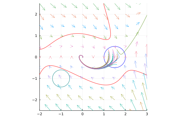
JuMP.primal_status(model)

FEASIBLE_POINT::ResultStatusCode = 1

Plot the phase plot with the 0-level set of the barrier function, and the boundary of the initial and unsafe sets

import OrdinaryDiffEqTsit5, Plots
function phase_plot(
    f,
    B,
    g₁,
    h₁,
    quiver_scaling,
    Δt,
    X0,
    solver = OrdinaryDiffEqTsit5.Tsit5(),
)
    Plots.plot()
    rx = range(-2, 3; length = 1000)
    ry = range(-2.5, 2.5; length = 1000)
    for (p, label, color) in
        ((h₁, "X₀", :blue), (g₁, "Xᵤ", :teal), (B, "B = 0", :red))
        Plots.contour!(
            rx,
            ry,
            (a, b) -> p(x[1] => a, x[2] => b);
            levels = [0.0],
            colorbar = false,
            aspect_ratio = :equal,
            label = label,
            linecolor = color,
        )
    end
    ∇(vx, vy) = [fi(x[1] => vx, x[2] => vy) for fi in f]
    ∇pt(v, p, t) = ∇(v[1], v[2])
    function traj(v0)
        tspan = (0.0, Δt)
        prob = OrdinaryDiffEqTsit5.ODEProblem(∇pt, v0, tspan)
        return OrdinaryDiffEqTsit5.solve(
            prob,
            solver,
            reltol = 1e-8,
            abstol = 1e-8,
        )
    end
    ticks = -5:0.5:5
    X = repeat(ticks, 1, length(ticks))
    Y = X'
    Plots.quiver!(
        X,
        Y,
        quiver = (x, y) -> ∇(x, y) / quiver_scaling,
        linewidth = 0.5,
    )
    for x0 in X0
        Plots.plot!(traj(x0), vars = (1, 2), label = nothing)
    end
    return Plots.plot!(xlims = (-2, 3), ylims = (-2.5, 2.5))
end

phase_plot(
    f,
    value(B),
    g₁,
    h₁,
    10,
    30.0,
    [[x1, x2] for x1 in 1.2:0.2:1.7, x2 in -0.35:0.1:0.35],
)

This page was generated using Literate.jl.