Mean Variance Portfolio Example

Consider the Markowitz portfolio selection problem, which allocates weights $x \in \mathbb{R}^n$ to $n$ assets so as to maximize returns subject to a variance limit $v_{\max}$:

\[\max_{x} \quad \mu^\top x \quad\text{s.t.}\quad x^\top \Sigma x \;\le\; v_{\max}, \quad \mathbf{1}^\top x = 1,\quad x \succeq 0,\]

where $\mu$ is the vector of expected returns, $\Sigma$ is the covariance matrix, and $x$ must sum to 1 (fully invest the budget). An efficient conic version of this problem casts the variance limit as a second order cone constraint:

\[\| \Sigma^{1/2} x \|_{2} \;\le\; \sigma_{\max}\]

where $\Sigma^{1/2}$ is the Cholesky factorization of the covariance matrix and $\sigma_{\max}$ is the standard deviation limit.

Practitioners often care about an \emph{out-of-sample performance metric} $L(x)$ evaluated on test data or scenarios that differ from those used to form $\mu$ and $\Sigma$. To assess the impact of the risk profile in the performance evaluation, one can compute:

\[\frac{dL}{d\,\sigma_{\max}} \;=\; \underbrace{\frac{\partial L}{\partial x}}_{\text{(1) decision impact}}\; \cdot\; \underbrace{\frac{\partial x^*}{\partial \sigma_{\max}}}_{\text{(2) from DiffOpt.jl}},\]

where $x^*(\sigma_{\max})$ is the portfolio that solves the conic Markowitz problem under a given risk limit.

Define and solve the Mean-Variance Portfolio Problem for a range of risk limits

First, import the libraries.

using Test
using JuMP
import DiffOpt
using LinearAlgebra
import SCS
using Plots
using Plots.Measures

Fixed data

Training data (in-sample)

Σ = [
    0.002 0.0005 0.001
    0.0005 0.003 0.0002
    0.001 0.0002 0.0025
]
μ_train = [0.05, 0.08, 0.12]

3-element Vector{Float64}:
 0.05
 0.08
 0.12

Test data (out-of-sample)

μ_test = [0.02, -0.3, 0.1]             # simple forecast error example

3-element Vector{Float64}:
  0.02
 -0.3
  0.1

Sweep over σ_max

σ_grid = 0.002:0.002:0.06
N = length(σ_grid)

predicted_ret = zeros(N)                 # μ_train' * x*
realised_ret = zeros(N)                 # μ_test'  * x*
loss = zeros(N)                 # L(x*)
dL_dσ = zeros(N)                 # ∂L/∂σ_max  from DiffOpt

for (k, σ_val) in enumerate(σ_grid)

    # 1) differentiable conic model
    model = DiffOpt.conic_diff_model(SCS.Optimizer)
    set_silent(model)

    # 2) parameter σ_max
    @variable(model, σ_max in Parameter(σ_val))

    # 3) portfolio weights
    @variable(model, x[1:3] >= 0)
    @constraint(model, sum(x) <= 1)

    # 4) objective: maximise expected return (training data)
    @objective(model, Max, dot(μ_train, x))

    # 5) conic variance constraint  ||L*x|| <= σ_max
    L_chol = cholesky(Symmetric(Σ)).L
    @variable(model, t >= 0)
    @constraint(model, [t; L_chol * x] in SecondOrderCone())
    @constraint(model, t <= σ_max)

    optimize!(model)

    x_opt = value.(x)
    println("Optimal portfolio weights: ", x_opt)

    # store performance numbers
    predicted_ret[k] = dot(μ_train, x_opt)
    realised_ret[k] = dot(μ_test, x_opt)

    # -------- reverse differentiation wrt σ_max --------
    DiffOpt.empty_input_sensitivities!(model)
    # ∂L/∂x   (adjoint)  =  -μ_test
    DiffOpt.set_reverse_variable.(model, x, μ_test)
    DiffOpt.reverse_differentiate!(model)
    dL_dσ[k] = DiffOpt.get_reverse_parameter(model, σ_max)
end

Optimal portfolio weights: [5.658840600212723e-6, 0.018882734866492903, 0.03907243442925988]
Optimal portfolio weights: [2.9615619528665894e-6, 0.03710076184578953, 0.07838697285156881]
Optimal portfolio weights: [3.991001332916834e-6, 0.0556573113824026, 0.11757663205482236]
Optimal portfolio weights: [2.8761053968294316e-5, 0.07467364263748005, 0.1565514737960362]
Optimal portfolio weights: [5.5336248609913934e-6, 0.09275568036215343, 0.19597607214341758]
Optimal portfolio weights: [6.045266093295765e-6, 0.11131252558506538, 0.23515581300531907]
Optimal portfolio weights: [6.794648070611909e-6, 0.12995866044115537, 0.2742970150707773]
Optimal portfolio weights: [3.223110683901139e-6, 0.14841388889233265, 0.31354555558295194]
Optimal portfolio weights: [5.691550122139736e-6, 0.1669701262219937, 0.3527322109736728]
Optimal portfolio weights: [7.023976971607716e-6, 0.18580227637112637, 0.39200323624664957]
Optimal portfolio weights: [4.62500582854471e-6, 0.2040057967872831, 0.4311552796865411]
Optimal portfolio weights: [5.727794364271045e-6, 0.222620949197694, 0.4703006360365732]
Optimal portfolio weights: [2.760617841535895e-6, 0.24122012282656582, 0.5094959120066633]
Optimal portfolio weights: [-4.011210802159187e-6, 0.2597179999164647, 0.5486899189726858]
Optimal portfolio weights: [2.483133946812592e-7, 0.278220419971934, 0.5879285717690754]
Optimal portfolio weights: [1.2656238263943147e-7, 0.2968306470378809, 0.627085999024414]
Optimal portfolio weights: [2.8403641386149958e-8, 0.3153827733669718, 0.6662793615646376]
Optimal portfolio weights: [-2.00064963638143e-6, 0.24354374836163056, 0.7564582014563547]
Optimal portfolio weights: [1.3793346961328554e-6, 0.170880138550446, 0.829113672335493]
Optimal portfolio weights: [1.12728226576089e-5, 0.11344879862059759, 0.8865392792745515]
Optimal portfolio weights: [-6.398848535048396e-9, 0.06232492177698422, 0.9376750967704776]
Optimal portfolio weights: [2.9505943490365626e-7, 0.014238262898225204, 0.9857589913469282]
Optimal portfolio weights: [-2.16150379865098e-5, -1.879168443294572e-5, 1.0000707785491552]
Optimal portfolio weights: [-1.306628516859309e-5, -1.3542094992647202e-5, 1.0000480370965048]
Optimal portfolio weights: [-1.3028821102573778e-5, -1.349888390969674e-5, 1.0000479074416557]
Optimal portfolio weights: [-1.333420459845848e-5, -1.3812256924856943e-5, 1.00004903592973]
Optimal portfolio weights: [-1.3095781403317063e-5, -1.3567686346371263e-5, 1.0000481547145872]
Optimal portfolio weights: [-1.3398025907370033e-5, -1.3878512620393833e-5, 1.0000492703600539]
Optimal portfolio weights: [-1.3439487711960188e-5, -1.392134256889034e-5, 1.000049423052066]
Optimal portfolio weights: [-1.3379282996105953e-5, -1.385946898906365e-5, 1.0000492007495632]

Results with Plot graphs

default(;
    size = (1150, 350),
    legendfontsize = 8,
    guidefontsize = 9,
    tickfontsize = 7,
)

(a) predicted vs realised return

plt_ret = plot(
    σ_grid,
    realised_ret;
    lw = 2,
    label = "Realised (test)",
    xlabel = "σ_max (risk limit)",
    ylabel = "Return",
    title = "Return vs risk limit",
    legend = :bottomright,
);
plot!(
    plt_ret,
    σ_grid,
    predicted_ret;
    lw = 2,
    ls = :dash,
    label = "Predicted (train)",
);

(b) out-of-sample loss and its gradient

plt_loss = plot(
    σ_grid,
    dL_dσ;
    xlabel = "σ_max (risk limit)",
    ylabel = "∂L/∂σ_max",
    title = "Return Gradient",
    legend = false,
);

plot_all = plot(
    plt_ret,
    plt_loss;
    layout = (1, 2),
    left_margin = 5Plots.Measures.mm,
    bottom_margin = 5Plots.Measures.mm,
)

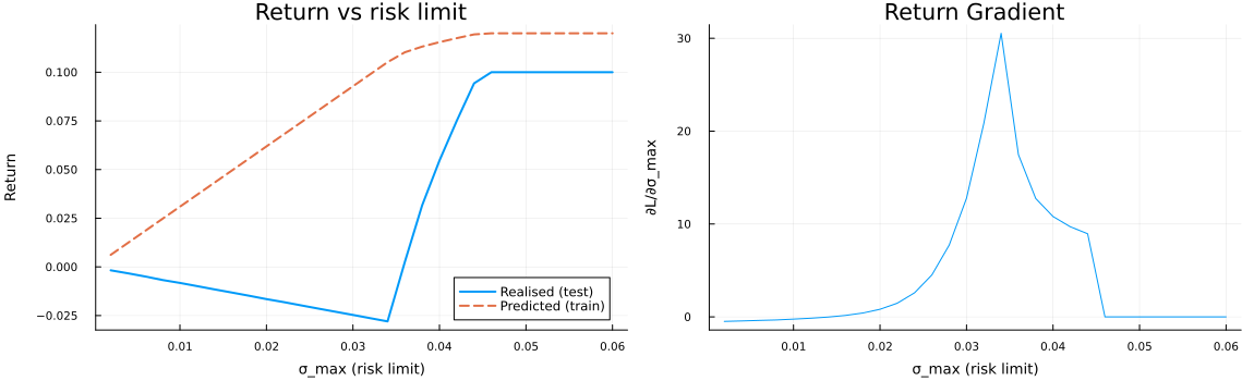
Impact of the risk limit $\sigma_{\max}$ on Markowitz portfolios. Left: predicted in-sample return versus realized out-of-sample return. Right: the out-of-sample loss $L(x)$ together with the absolute gradient $|\partial L/\partial\sigma_{\max}|$ obtained from DiffOpt.jl. The gradient tells the practitioner which way—and how aggressively—to adjust $\sigma_{\max}$ to reduce forecast error; its value is computed in one reverse-mode call without re-solving the optimization for perturbed risk limits.

This page was generated using Literate.jl.